
GUIDE · GO PERFORMANCE INVESTIGATION · 12 MIN READ
Go allocation profiling: pprof, escape analysis and benchmarks
Investigate Go allocations with alloc_space and inuse_space profiles, compiler escape analysis and equivalent formatter benchmarks. Includes tested downloadable code.
Edition: · Practical guide. Added to the archive on the publication date above. Sources and worked examples below.

Start with a question that a profile can answer
A Go endpoint becomes expensive after a product change. Its latency increases, allocation charts rise, and somebody proposes replacing every fmt call with a hand-written encoder. That might improve the endpoint, but it might also consume a week while the actual problem remains an unbounded result cache. Before changing code, decide whether the incident concerns allocation traffic, retained memory, CPU time, latency, or a combination of them.
These are different optimization targets. Allocating less over an interval can reduce pressure on the runtime without reducing the long-lived cache. Removing retained objects can reduce the live heap while leaving request-level allocation traffic unchanged. Faster formatting can save CPU even when every returned string still needs an allocation. A useful investigation keeps those claims separate and tests the behavior that users actually receive.
This guide walks through an original memory-profile experiment and a pair of equivalent formatting benchmarks. The lab uses native Go 1.27.3 on darwin/arm64, Apple M4, with GOMAXPROCS two. It includes source, tests, raw observations and commands. These local observations are a reproducible learning exercise, not a claim about every service or the execution characteristics of GopherForge's app sandbox.
Understand allocation traffic and retained memory separately
Imagine a worker that creates two thousand temporary blocks while keeping a small sample of them in a result. Almost all of its allocation traffic can disappear from the live heap after collection. A different worker might allocate very little during the same observation window while retaining a large cache created earlier. Looking only at one memory chart cannot distinguish those programs.
The runtime/pprof documentation describes the heap profile and its relationship to completed garbage collection. The profile includes sample types that let tools examine allocation history and retained allocations. Use alloc_space to investigate sampled allocated bytes and inuse_space to investigate sampled bytes still in use at the profile's collection boundary. Neither view is a complete ownership graph.
The allocation stack answers where storage was created. It does not necessarily identify the field, queue, closure or registry that currently owns it. A parser can appear prominently in a retained-memory profile because another component stores its results indefinitely. Deleting the parser's allocation would change the feature; changing the retention policy may solve the actual incident.
Read the companion heap-graph investigation when an apparently small result holds a large backing allocation. Read the GC controls lab when collection pressure is being confused with application ownership.
Construct a profile whose expected outcome is known
Our profile mode allocates 2,048 blocks of 64 KiB, for 128 MiB of application payload allocation. It keeps every 128th block, so sixteen blocks remain reachable: exactly one MiB of retained payload. Separate helper functions name the retained and temporary paths. The experiment clears its temporary reference and requests completed collections before writing the profile.
That design gives the profile an independently checkable expectation. Allocation traffic should be dominated by the temporary path, while retained application payload should be associated with the retained path. The program also uses runtime.KeepAlive after the observation boundary so that its retained result remains relevant throughout the measurement.
go build -o memlab ./cmd/memlab
./memlab -mode profile -out heap.pprof
go tool pprof -top -sample_index=alloc_space ./memlab heap.pprof
go tool pprof -top -sample_index=inuse_space ./memlab heap.pprof
The experiment sets the memory-profile sampling rate to 64 KiB before creating its workload. This improves the detail available for a small demonstration, but it changes profiling overhead and does not turn a sampled profile into an exact allocation ledger. Keep the chosen rate beside the results. Do not copy the setting into a production process without considering the observation cost.
Read the two profile views without inventing precision
In the recorded run, pprof's alloc_space report printed about 127.91 MB total. The temporary churn helper accounted for 126.85 MB and the retained helper for 0.99 MB. The inuse_space report printed about 1,077.47 kB total, with 1,012.46 kB attributed to the retained helper. These are the units and sampled estimates printed by pprof, rather than exact byte counts reconstructed from the source.
| Question | Profile view | Main application allocation site in this run |
|---|---|---|
| Where did allocation traffic originate? | alloc_space | churnBlock: 126.85 MB |
| Which allocated payload remains represented? | inuse_space | retainedBlock: 1,012.46 kB |
| How much payload did the program intentionally retain? | Source-level invariant | 16 × 64 KiB = 1 MiB |
The Go performance guidance explains the sampling nature of memory profiles. Small runtime allocations and statistical estimation help explain why the printed profile is not identical to the source-level invariant. The reliable conclusion is the separation of temporary traffic from retained payload, not a promise that every run prints those same decimals.
An important negative conclusion follows: a quiet temporary allocation site in inuse_space does not prove that site is cheap. It may still create substantial allocation traffic and CPU work. Likewise, a prominent retained site does not prove a leak. Retention may be intentional and correctly bounded. Follow the profile with an ownership and workload review.
Capture profiles at comparable lifecycle boundaries
An incident investigation needs to state when the profile was captured. Was the cache cold or warm? Had requests finished? Was a collection explicitly requested? Was the process still admitting work? A profile taken during startup cannot be compared casually with one taken after several hours of accumulated application state.
For a batch service, choose boundaries such as before the batch, after a representative batch, and after results have been released. For a long-running endpoint, record request volume, payload sizes, active operations and cache entries around the observation window. If the workload changes, a larger allocation total may reflect more completed useful work rather than a regression.
The Go diagnostics guide provides a broader map of profiling tools. Use CPU profiles for CPU attribution and memory profiles for their defined allocation views. A heap profile cannot establish tail latency, and an allocation benchmark cannot establish how an entire service behaves under concurrent load.
If you expose the net/http/pprof handlers, keep diagnostics on an appropriately restricted management surface. Profiles can contain implementation details and observations about a running service. The downloadable lab writes a local profile file instead, making the learning exercise independent of network configuration or a public diagnostics endpoint.
Compare implementations that return the same result
The second experiment asks a narrower question: can a small formatter produce the same string with less execution time? The baseline uses fmt.Sprintf. The alternative uses strconv append operations and converts the completed buffer to a string. Both return a value that callers can retain independently.
func FormatEvent(id uint64, active bool) string {
    return fmt.Sprintf("id=%d active=%t", id, active)
}

func AppendEvent(id uint64, active bool) string {
    buf := make([]byte, 0, 48)
    buf = append(buf, "id="...)
    buf = strconv.AppendUint(buf, id, 10)
    buf = append(buf, " active="...)
    buf = strconv.AppendBool(buf, active)
    return string(buf)
}
The fmt reference defines the formatting operations used by the baseline. The strconv reference defines the typed append operations used by the alternative. This example has a deliberately small output contract. It is not a replacement for general formatting, localization, JSON escaping or arbitrary user-controlled templates.
Before timing either function, the tests compare their results for zero, several ordinary identifiers, the maximum uint64 value, and both boolean values. A faster function that drops a space, changes a sign convention or returns mutable shared storage is not an equivalent optimization. The output contract determines what the benchmark is allowed to change.

Use a benchmark harness that preserves useful work
The benchmark fixture uses the identifier 123456789 and the value true. It assigns the returned string to a package-level sink and reports allocations. Both implementations use the same fixture, result destination and loop structure. Setup stays outside the timed loop.
var result string

func BenchmarkAppend(b *testing.B) {
    b.ReportAllocs()
    for b.Loop() {
        result = AppendEvent(123456789, true)
    }
}
The testing.B.Loop documentation describes its timing and compiler-preservation behavior. Use its supported loop form rather than assuming any hand-written wrapper has equivalent properties. The global sink also makes the intended observable result explicit in this example.
GOMAXPROCS=2 go test -run '^$' \
  -bench 'Benchmark(Format|Append)$' \
  -benchmem -benchtime=150ms -count=5
Record the toolchain and machine with the output. The Go testing flags define the benchmark controls. Repeated runs help reveal variation, but five short repetitions on one machine do not establish a production performance distribution. Change the fixture deliberately when evaluating different identifier sizes, output lengths or workload mixes.
A faster formatter can have the same allocation count
The five recorded baseline timings were 51.91, 46.51, 47.36, 45.76 and 45.97 ns/op. The append version produced 12.50, 12.36, 12.19, 12.09 and 12.12 ns/op. Their medians were 46.51 and 12.19 ns/op respectively. Every recorded run reported 24 B/op and one allocation per operation for both implementations.
| Implementation | Median of five runs | Reported bytes per operation | Reported allocations per operation |
|---|---|---|---|
| fmt.Sprintf | 46.51 ns/op | 24 | 1 |
| strconv append operations | 12.19 ns/op | 24 | 1 |
This is useful evidence for a specific CPU-oriented improvement in a specific fixture. It is not evidence that the alternative removed the returned string's allocation. The benchmark records both dimensions precisely because the attractive headline, faster formatting, could otherwise be mistaken for a different claim, less allocation traffic.
Do not generalize the observed timing ratio to whole requests. If formatting accounts for a small fraction of endpoint CPU, even a substantial improvement there may barely affect end-to-end latency. A service waiting on its database will not become several times faster merely because this isolated formatter does. Use a representative CPU profile to estimate whether the local improvement addresses a meaningful cost.
Use escape analysis to explain, not replace, measurements
Build the package with compiler diagnostics and inspect the messages for the actual source version. The compiler documentation describes the diagnostic flag. Decisions can change with inlining, surrounding code, compiler updates and how the result is used.
go build -gcflags=-m=2 .For the recorded Go 1.27.3 build, the compiler reported that make([]byte, 0, 48) in AppendEvent did not escape and that string(buf) escaped to the heap. Those diagnostics are consistent with the benchmark's single result allocation. The complete diagnostic output is included with the experiment, so the explanation can be checked against the selected compiler rather than remembered as a permanent language rule.
Do not count every line containing escapes as one executed allocation. A diagnostic describes an analysis decision at a source location, not a runtime event counter. A path may execute conditionally, a call may be inlined differently, and surrounding optimization can change the final behavior. Use benchmark allocation counts and profiles to measure the built workload.
The stack-and-heap lesson and escape-analysis interview guide cover the broader reasoning. The practical habit is simple: form a hypothesis with diagnostics, then verify its effect with equivalent behavior and actual measurements.
Avoid changing ownership to win a benchmark
A tempting next step is to return a view into a reusable buffer. That can reduce a local allocation count while allowing a later call to overwrite an earlier result. The benchmark may improve precisely because the implementation stopped providing independent ownership. Such a change needs a different API contract, not a celebratory allocation chart.
If callers can consume bytes synchronously before the next mutation, an append-to-caller-buffer API can be appropriate. If callers store the returned value, independent storage may be necessary. A zero-copy technique is valuable only when its lifetime and mutation restrictions fit the application. Make those restrictions visible in names, documentation and tests.
The buffer and pool ownership guide explains why reuse requires a clear handoff. Pooling also has its own memory and concurrency tradeoffs. Reusing an oversized buffer can preserve capacity long after a small request ends, while incorrect reuse can corrupt output across operations.
Treat a changed ownership contract as an architectural decision. Test that a previous result remains valid after a subsequent call, and test concurrent usage if the API promises it. Allocation reduction is not a sufficient acceptance criterion when the feature depends on stable independently owned results.
Check the workload level before rolling out a local win
A benchmark operation and a user request are not necessarily the same unit of work. An endpoint might format one event, a thousand events, or no events on its common path. Record that relationship before translating nanoseconds per operation into a capacity estimate. Also ask whether the formatter is on the critical path or runs after the response has already completed.
Consider an illustrative calculation, not another measurement from this lab. If formatting consumes five percent of request CPU and a replacement makes that component four times faster, the total CPU reduction is only 3.75 percent under otherwise identical conditions. The remaining ninety-five percent has not changed. Waiting time, contention and request concurrency introduce additional effects that this arithmetic does not model. This helps explain why a clear microbenchmark improvement can produce a modest service-level result.
Build a small fixture matrix before rollout: short and maximum-width identifiers, both boolean values, ordinary and unusually large batches, and the actual destination used by the caller. Keep the correctness suite independent from the timing suite. A rare input can be essential to correctness even when it should not dominate a representative timing fixture.
Finally, compare useful completed operations under equivalent demand. A deployment that reports fewer allocated bytes because it rejected more requests has changed throughput as well as memory use. Preserve acceptance rates, error rates, payload distribution and latency beside resource measurements. Those observations let the team decide whether the local optimization improved the feature that motivated the investigation.
Build a repeatable optimization decision
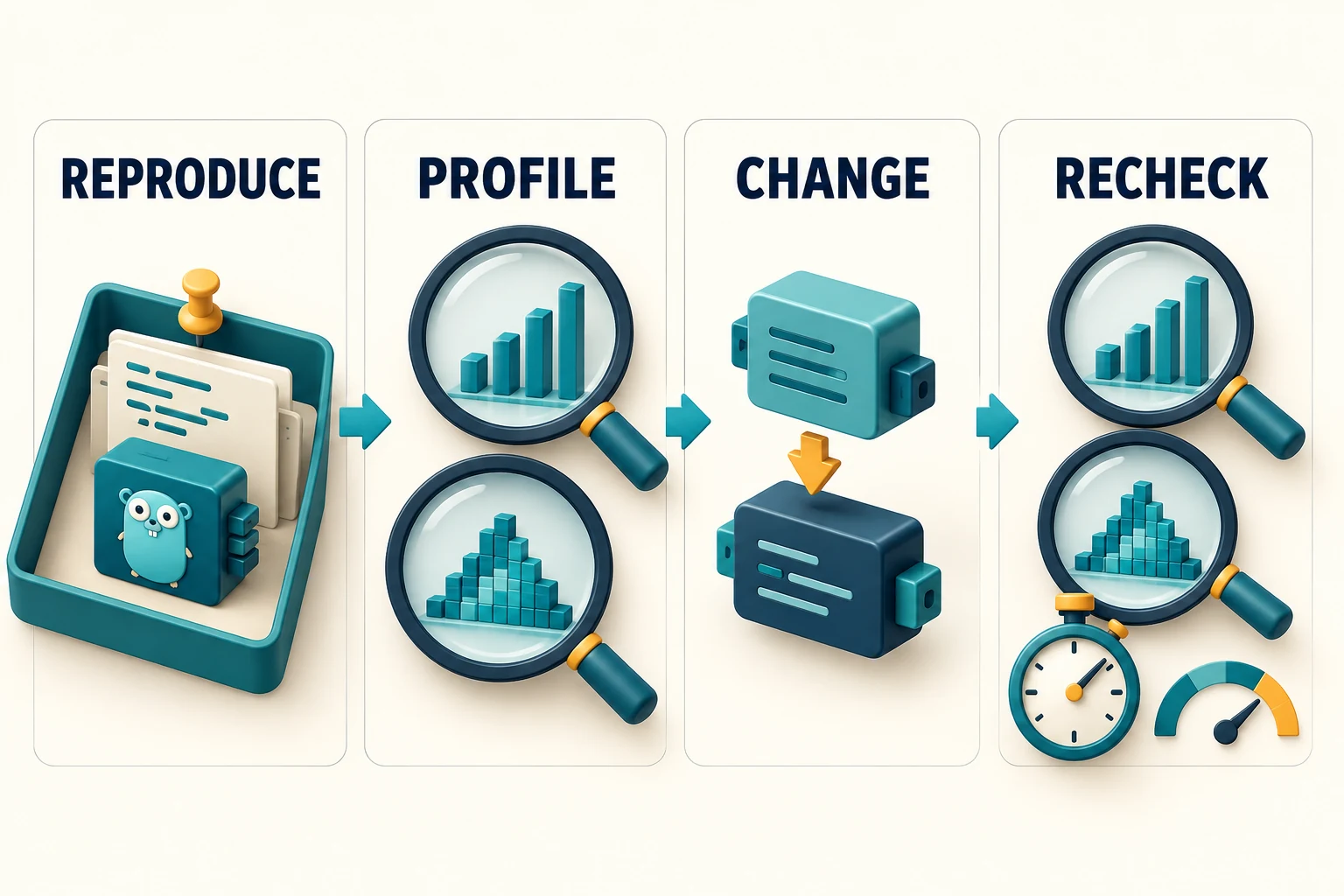
An actionable performance change includes the original symptom, a representative fixture, an explicit result contract, a baseline, the modified implementation and a recheck of correctness and resources. Preserve raw outputs. Explain which dimension improved and which dimensions were unchanged or not measured. Include a rollback path if the change affects a production service.
The lab tests also support deliberately broken variants as negative controls. Returning an aliased prefix must fail the independence test. Removing a separator must fail the formatting equivalence test. Disconnecting a graph node must fail structural validation. These checks make sure the test suite can reject meaningful defects rather than merely run successfully against its own implementation.
Download the original memory lab, tests and raw observations. Start with the profile modes, reproduce the formatting comparison, then change one fixture at a time. Keep native desktop measurements separate from app-sandbox behavior and from production service limits.
Continue with profiles and leak investigation, GC budgets, and the companion heap ownership article. A strong optimization report does not promise that allocations are universally bad. It shows which cost mattered, why the change preserves behavior, and what the measured evidence actually supports.
Primary sources & editorial method
We checked these primary references on 29 October 2026. Release facts are attributed; recommended workflows and examples are GopherForge analysis. Illustrations are conceptual, not vendor screenshots or benchmarks.