
GUIDE · GO GARBAGE COLLECTION · 12 MIN READ
Go garbage collection: a practical GOGC and GOMEMLIMIT lab
Understand Go garbage collection with tested GOGC and GOMEMLIMIT experiments, live-heap accounting, allocation traffic and a reproducible memory-budget workflow.
Edition: · Practical guide. Added to the archive on the publication date above. Sources and worked examples below.

Start with the symptom, not a collector setting
A Go service with rising memory use does not necessarily have a garbage-collector problem. It may be retaining a larger cache, admitting more concurrent requests, buffering larger payloads, or keeping abandoned work alive. Conversely, a service with a stable live heap can spend substantial CPU repeatedly collecting short-lived allocations. Those incidents require different changes even when the same memory graph appears in both incident reports.
Imagine a document-processing API that reads an input, constructs several temporary representations, and keeps a small result in a cache. After traffic increases, CPU and memory both rise. Before changing GOGC, ask which quantity changed: requests per second, allocated bytes per request, retained bytes per result, concurrent operations, or the size of the cache. A collector cannot decide which cached documents the business no longer needs, and it cannot make an unbounded queue into a bounded one.
This guide combines a short model of Go GC controls with an original, deliberately small experiment. The measurements were made with native Go 1.27.3 on darwin/arm64, Apple M4, with GOMAXPROCS set to two. They are useful for understanding relationships, not choosing production defaults. The complete program, raw observations and commands are downloadable below. The GC-budget lesson provides a shorter introduction; here we focus on turning observations into a defensible engineering decision.
Keep four memory quantities separate
Begin with live heap, allocation traffic, runtime-managed memory and operating-system memory. Live heap describes objects still reachable after collection. Allocation traffic describes memory requested over an interval, including objects that have already become garbage. Runtime-managed memory includes more than the live heap. A process's operating-system footprint also includes memory outside the collector's direct accounting.
These quantities answer different questions. A temporary parser can allocate hundreds of megabytes while retaining almost nothing after a batch finishes. A cache can allocate little during a quiet interval while holding a large existing object graph. A service can release Go objects without immediately showing the same reduction in an operating-system residency chart. A useful dashboard should not label all of those measurements simply as memory.
The runtime memory-statistics reference defines the individual fields. Keep their names in your measurements so that another engineer can reproduce the interpretation. For example, TotalAlloc is a cumulative counter, while HeapAlloc is a current heap measurement; comparing them as though both described current retained data leads to misleading conclusions.
Our document API should therefore record at least the input size, concurrency, allocation traffic and retained state alongside latency. Without that workload context, a change in the memory chart may reflect a different amount of useful work rather than an improvement or regression in memory management.
Use the GOGC model to reason about headroom
The official Go GC guide describes a simplified relationship between the live heap, roots and the next heap target. In that model, the target is the live heap plus additional room proportional to the live heap and roots, scaled by GOGC. The model explains a tradeoff; it is not a promise about exact RSS, a fixed allocation size or every point in a concurrent collection cycle.
approximate target = live heap + (live heap + roots) × GOGC / 100A larger GOGC generally permits more allocation headroom between collections. A smaller value generally asks the runtime to collect more frequently. Neither choice changes whether an application still owns a particular object. If the cache permanently retains twice as much useful or useless data, changing the collector percentage does not remove that ownership.
Use the model as a hypothesis generator. If allocation traffic is high but retained state is small, investigate allocation sites. If retained state grows with cache entries, investigate the cache policy. If a workload has many pointer-rich objects, consider the shape and amount of data the collector must inspect, not only total bytes. The companion heap-graph investigation makes that distinction concrete.
A memory limit is not a hard process-size guarantee
GOMEMLIMIT and runtime/debug.SetMemoryLimit provide a soft limit for memory managed by the Go runtime. The SetMemoryLimit documentation defines its accounting in terms of Sys minus HeapReleased. It also identifies excluded sources such as memory managed outside Go. Therefore setting the runtime limit equal to a container's hard memory allowance does not establish a complete safety margin.
Budget for the whole process and its environment. Depending on the program, that can include native libraries, explicit mappings, binary pages and operating-system overhead. Measure the actual deployment instead of subtracting an arbitrary percentage from a number copied out of a manifest. If the program already needs nearly all available memory for reachable objects, an aggressively low soft limit may increase collection pressure without creating the missing capacity.
Treat the container allowance and runtime control as related but separate decisions. A useful configuration record states the hard environment limit, expected live data, measured non-heap overhead, transient work and operational reserve. It also states what the service does when demand exceeds that budget: reject work, reduce concurrency, evict entries, or move work elsewhere.
Our fictional API might first limit concurrent document conversions and reject oversized inputs. That changes the amount of memory the application asks to own. Only after those boundaries are explicit does collector tuning become an understandable adjustment rather than an attempt to hide an unbounded workload.
Build an experiment with a narrow claim
The downloadable lab holds one twelve-MiB byte buffer alive and repeatedly allocates 512 blocks of 512 KiB: 256 MiB of allocation traffic. A completed collection establishes the starting point before the allocation loop. The program records collection counts and the heap goal at the end of that loop, then collects again before measuring retained memory.
Each setting runs in a fresh process three times. The runtime version, architecture, GOMAXPROCS, environment settings and raw JSON are recorded. The large buffers contain bytes rather than pointers to other heap objects. That matters: this experiment is intentionally not a model of a pointer-rich object cache, a concurrent web service, or a memory-intensive native library.
go build -o memlab ./cmd/memlab
GOGC=50 ./memlab -mode gc
GOGC=100 ./memlab -mode gc
GOGC=200 ./memlab -mode gc
GOGC=200 GOMEMLIMIT=32MiB ./memlab -mode gc
Before comparing runs, clear an inherited GOMEMLIMIT when testing the cases without a limit. The lab runner does this explicitly. An unnoticed environment setting can otherwise make two apparently different GOGC runs obey the same effective constraint. The goal is to understand what changed, not merely collect a row of numbers that looks scientific.
What this local experiment actually showed
The following table uses medians across three fresh processes. The heap-goal column is the observed target at the end of the allocation loop, not peak memory use or a guaranteed cap. Approximate MiB values are conversions of recorded byte counts.
| GOGC | GOMEMLIMIT | Collections during allocation loop | End-of-loop heap goal |
|---|---|---|---|
| 50 | not set | 39 | 19.90 MiB |
| 100 | not set | 19 | 26.60 MiB |
| 200 | not set | 8 | 55.00 MiB |
| 200 | 32 MiB | 21 | 25.88 MiB |
The collector ran less frequently when more headroom was allowed in this workload. Adding a soft limit constrained that relationship. After an explicit final collection, every case still retained roughly the same twelve-MiB application buffer. No setting made that reachable buffer disappear.
The loop's measured durations were only a few milliseconds. That is too short and narrow a test to establish a production performance ranking. We deliberately do not turn them into a claim that one setting makes a service faster. Background activity, allocator behavior and the synthetic workload matter. Likewise, the observed targets do not need to equal a formula evaluated from the final heap: the pacer uses collection history and the runtime is operating concurrently.
The useful result is the relationship between headroom, collection frequency and unchanged live ownership. For production, repeat the experiment with representative object lifetimes, concurrency and latency measurements before selecting a setting.

Distinguish collector work from application allocation work
A CPU increase can involve allocating and initializing objects, tracing reachable objects, reclaiming memory, synchronization, or unrelated application work. A single GC-cycle count cannot identify which part dominates. A lower number of collections is not automatically a lower end-to-end cost, just as fewer database queries do not automatically mean a faster endpoint.
Use CPU profiles and runtime observations together. The diagnostics guide describes the available profiling tools. A useful investigation follows the allocation site back to the operation that creates demand: a temporary conversion, a per-item map, a repeated string representation or an unnecessarily retained response buffer.
For the document API, compare equivalent outputs. Removing an allocation by dropping a validation step is not an optimization of the same behavior. Reusing a mutable buffer without giving callers independent ownership can improve a microbenchmark while corrupting concurrent responses. A performance change needs a correctness test as well as a resource measurement.
Our allocation-profiling lab includes a revealing counterexample: a faster formatting implementation that still performs the same number of result allocations. That is a useful improvement in one dimension, but it is not evidence that GC traffic disappeared. Separate the claim you measured from the claim you hoped to prove.
Measure roots and scannable data deliberately
A large byte buffer and a collection of small pointer-rich nodes can occupy similar numbers of bytes while presenting different tracing work. Roots also matter: stacks and globals can keep object graphs reachable. Increasing the number of concurrent operations can therefore change both retained state and the set of roots the runtime must consider.
The runtime/metrics catalog exposes measurements for scannable heap space, stack scanning and globals. Those measurements have different definitions and should not all be interpreted as the number of bytes actually visited during an arbitrary request. Preserve the metric names and read the matching toolchain's descriptions before constructing a ratio.
For example, /gc/scan/heap:bytes describes scannable heap space. It is not a direct count of pointer edges, a heap-depth limit or a duration. A large pointer-free payload can contribute heavily to live bytes without contributing the same amount of pointer-bearing content. That does not make it free: it still occupies memory and participates in allocation and object bookkeeping.
A practical cache review should therefore ask what each entry retains, how entries reference each other, and how the cache is bounded. The reachability lesson is a better starting point for that review than searching for a collector flag that promises to ignore application-owned objects.
Avoid making manual collection part of every request
The lab calls runtime.GC to establish observation boundaries. That is an experimental control, not a recommendation to force collection after each API request. A manually imposed collection can add work and change the behavior you are trying to observe. It can also distract from the actual problem: the application still retaining the wrong objects or producing avoidable allocation traffic.
Similarly, a single low heap measurement immediately after a forced collection does not describe a workload's peak usage. A service may grow again during the next burst, and the operating system may account for released and reserved memory differently from the heap statistic you sampled. Collect a time series around meaningful workload transitions.
For a batch processor, compare memory before work, during a bounded peak, after completion and after a quiet period. State whether a collection was explicitly requested at each boundary. For a long-running service, prefer a representative observation window and correlate memory with admitted work, completed work and cache size.
If forced collection is part of a justified operational procedure, document why, how frequently it runs and what outcome it is expected to change. Treat it as a measured intervention with costs, not a universal cleanup button whose successful return proves that the process is now small.
Turn tuning into a controlled rollout
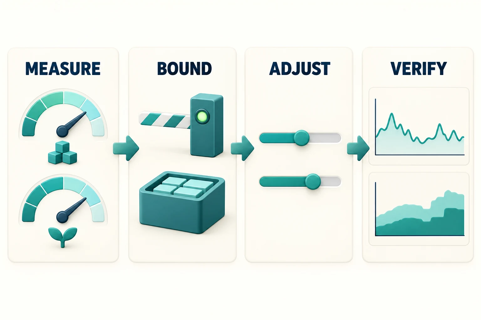
Change one variable at a time. First establish the workload envelope and correctness tests, then capture a baseline. Apply a collector setting to a limited deployment slice and compare useful completions, latency, runtime memory and collection pressure under equivalent demand. Keep a rollback value and a stopping condition.
Do not compare a quiet weekday baseline with a busy release window and attribute the whole difference to GOGC. Note payload distribution, cache warmup, replica count and background jobs. A change that works with a cold cache may behave differently after the live object graph has grown. A setting that looks good on a native desktop may be inappropriate in a constrained container or an app sandbox.
Use the service's own availability objective. If a lower memory allowance creates sustained collection pressure and harms request completion, that is not a successful memory optimization merely because a graph has a lower ceiling. Conversely, accepting more memory to reduce CPU may be reasonable only if the deployment actually has that headroom across all replicas.
The lesson from bounded work applies directly: capacity decisions belong to the application and deployment, not only to the collector. A collector policy should support those boundaries, and the rollout should verify that the intended business work still completes.
Keep a reproducible memory budget beside the service
A useful handoff includes the selected toolchain, workload shape, live-data expectations, input and concurrency limits, collector settings, raw measurements and a repeatable command. It also explains what was not measured. Our experiment records Go-managed memory and collection behavior; it does not measure production RSS, tail latency, native-library memory or every allocation pattern a real application may produce.
Download the original memory lab, tests and measurement data. The archive includes the GC workload, graph-shape and retention modes, formatting benchmarks and a README. The measurements are small local observations with their methodology attached, not a benchmark leaderboard.
Continue with GC interview preparation, stack and heap ownership, and the companion heap-graph investigation. When memory behavior becomes confusing, return to the same sequence: identify the owner, bound the work, measure the relevant quantity, change one decision, and verify the outcome. That sequence remains useful even when a future Go release changes the collector's implementation details.
Primary sources & editorial method
We checked these primary references on 29 October 2026. Release facts are attributed; recommended workflows and examples are GopherForge analysis. Illustrations are conceptual, not vendor screenshots or benchmarks.